This project is an implementation of the ground-breaking 3D volumetric reconstruction work by Ben Mildenhall, NeRF and was written in Python3 and made use of the following libraries- PyTorch, NumPy, Hydra, and Matplotlib. This project was implemented as a part of my Spring 2023 course at CMU, Learnig for 3D Vision, taught by Prof. Shubham Tulsiani.

Volume Reconstruction

Ray Sampling

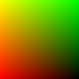
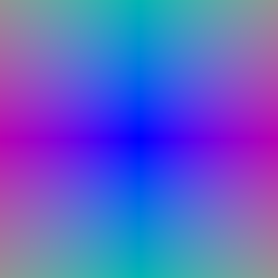
First part in the process to generate a NeRF is to desgn a ray sampler, capable of producing 3D rays in the world space, from a given set of image co-ordinates. This is done by generating a normalized meshgrid over the image dimensions, using Pytorch.meshgrid and using this to project rays into 3D space. These rays, currently in camera space, are then transformed into world space using appropriate camera extrinsics. The image below shows an exmaple of a meshgrid and the resulting rays visualized from the origin location.

The left figure shows a visualization of the image coordiantes. The right image shows a visualization of the projected rays from the origin

Point Sampling

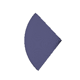
The second step involves sampling points, using the rays generated in the previous section. Points are sampled along the rays generated, at stratified intervals, up until a maximum threshold. This gives us a semicircular point cloud of samples along the rays, which can be seen visualized in the image below.

Sampled points in a bundle of rays

Volume Rendering

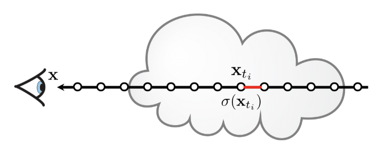
Now, a volume rendering function is designed, which would take input the sampled points defined in the previous section, and an implicit volume function for an object and use the transmittance equations defined below to produce a volume rendering for that object. The equations can be underestood from the figure below which shows a point sampling inside an object. The first equation is a recursive equation, that calulates the emission (color) for the segment i, shown in red below. The second equation calculates the transmittance of this segment with respect to the point-of-view (eye in the figure), based on the object absorption and emission coefficients. Please visit this page for detailed explanation on transmittance calculations in volume rendering

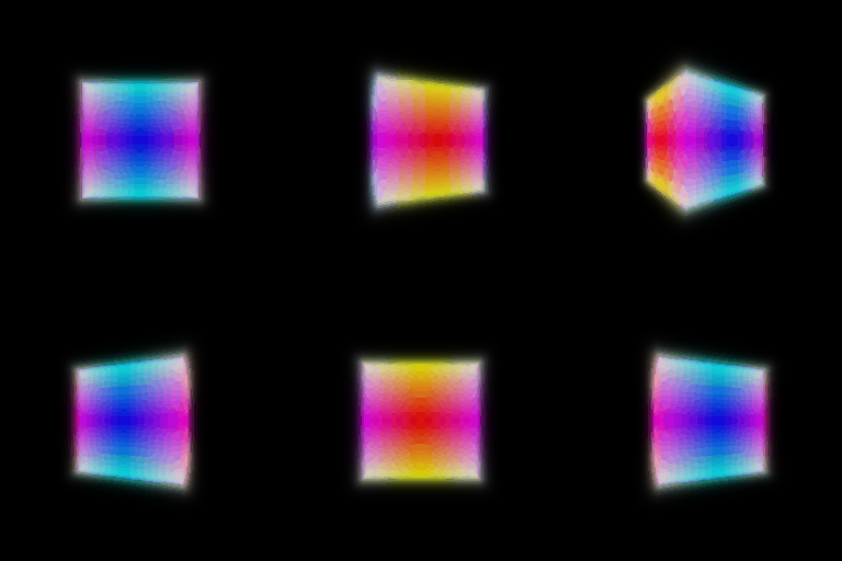
$$ L(x,w)= \sum_{i=1}^{N} T(x, x_{t_i})(1 - e^{-\sigma_{t_{i}} \Delta t_i }) L_e(x_{t_i}, w) $$ $$ T(x, x_{t_i}) = T(x, x_{t_{i-1}})e^{-(\sigma_{t_{i-1}} \Delta t_{i-1})} $$

A sample rendering using this renderer, for a cube is shown in the animation below.

Cube render using the Volume Renderer

Designing NeRF

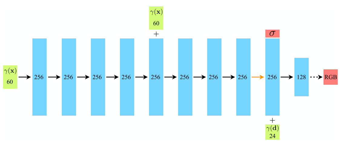
A neural radiance field is a neural network used to approximate the implicit function for any given object. It is trained on multiple images of this object and is capable of producing continuous volume renders. The multi-layered perceptron (MLP) network used by me for this purpose is shown below

MLP used for NeRF

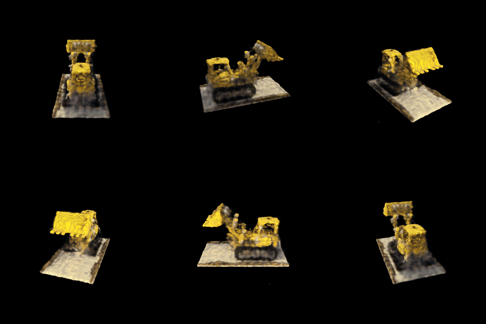
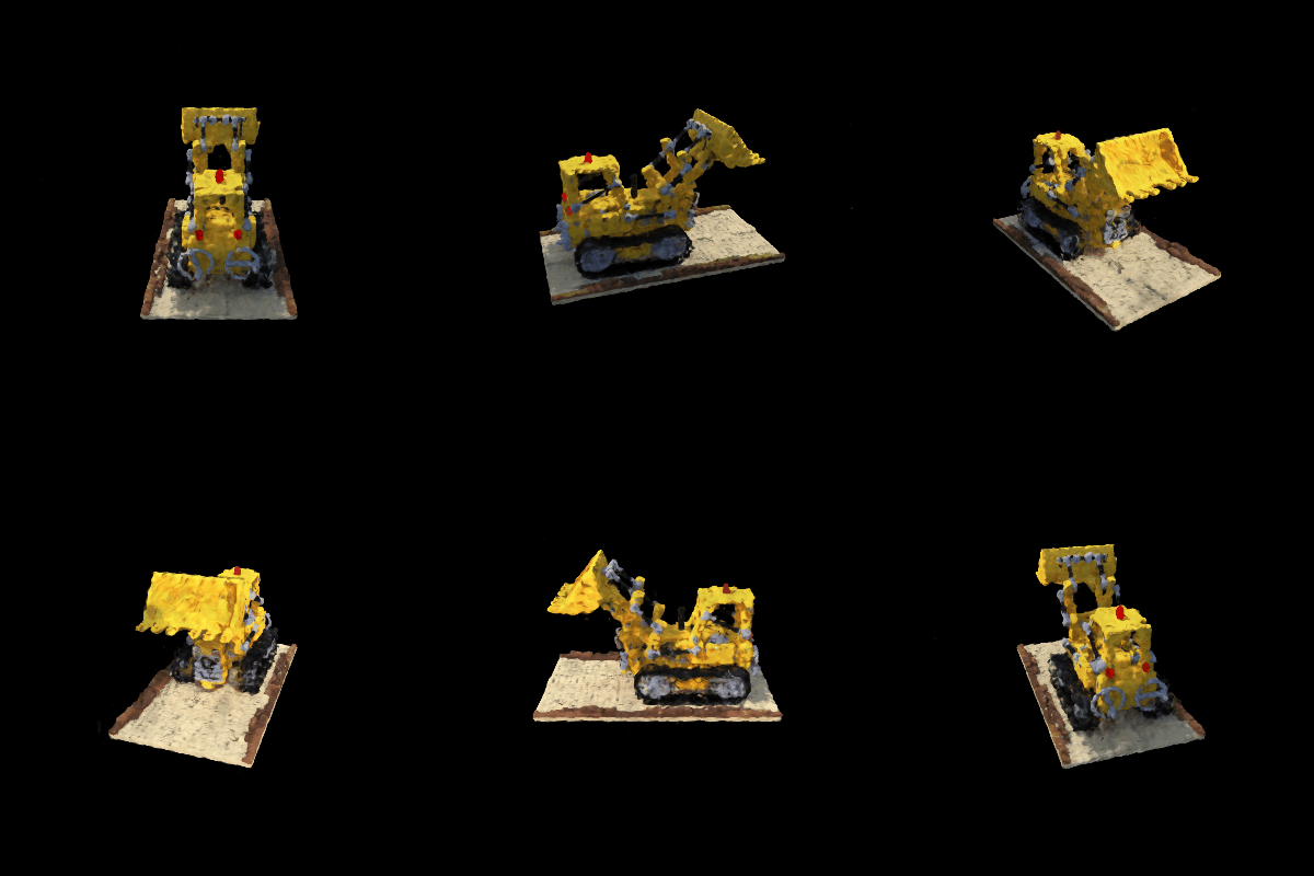
This MLP was trained on the multi-view images of a bulldozer. The hyperparamters used for this training are listed in the table below. The results of the volume rendering can be seen in the image below.

Hyperparameter	Value
Learning rate	1e-4
Epochs	250
Batch Size	1024
Number of Sampled Rays	32768
Number of Points per Ray	128
Image Resolution	600X600

NeRF volume rendering results for bulldozer

NeRF progression through training. From left to right - 50 epochs, 100 epochs, 250 epochs

Surface Reconstruction

The implementation of NeRF was extended to include Surface Reconstruction, using Neural Implicit Surfaces. Here, we implement a Neural SDF which is basically an approximation of the signed distance function (SDF) for any object using a neural network. SDF is the signed orthogonal distance of a given point to the boundary of an object. The sign determines whether the point lies inside or outside the boundary. The function has positive values for points inside the boundary.